Due to the massive growth of social media in the last decade, it has become a rage among data enthusiasts to tap into the vast pool of social data and gather interesting insights like trending items, reception of newly released products by society, popularity measures to name a few.
We are continually evolving PriceWeave, which has the most extensive set of offerings when it comes to providing actionable insights to retail stores and brands. As part of the product development, we look at social data from a variety of channels to mine things like: trending products/brands; social engagement of stores/brands; what content “works” and what does not on social media, and so forth.
We do a number of experiments with mining Twitter data, and this series of blog posts is one of the outputs from those efforts.
In some of our recent blog posts, we have seen how to look at current trends and gather insights from YouTube the popular video sharing website. We have also talked about how to create a quick bare-bones web application to perform sentiment analysis of tweets from Twitter. Today I will be talking about mining data from Twitter and doing much more with it than just sentiment analysis. We will be analyzing Twitter data in depth and then we will try to get some interesting insights from it.
To get data from twitter, first we need to create a new Twitter application to get OAuth credentials and access to their APIs. For doing this, head over to the Twitter Application Management page and sign in with your Twitter credentials. Once you are logged in, click on the Create New App button as you can see in the snapshot below. Once you create the application, you will be able to view it in your dashboard just like the application I created, named DataScienceApp1_DS shows up in my dashboard depicted below.

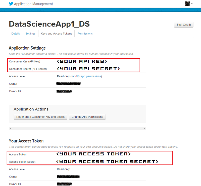
On clicking the application, it will take you to your application management dashboard. Here, you will find the necessary keys you need in the Keys and Access Tokens section. The main tokens you need are highlighted in the snapshot below.
I will be doing most of my analysis using the Python programming language. To be more specific, I will be using the IPython shell, but you are most welcome to use the language of your choice, provided you get the relevant API wrappers and necessary libraries.
Installing necessary packages
After obtaining the necessary tokens, we will be installing some necessary libraries and packages, namely twitter, prettytable and matplotlib. Fire up your terminal or command prompt and use the following commands to install the libraries if you don’t have them already.
Creating a Twitter API Connection
Once the packages are installed, you can start writing some code. For this, open up the IDE or text editor of your choice and use the following code segment to create an authenticated connection to Twitter’s API. The way the following code snippet works, is by using your OAuth credentials to create an object called auth that represents your OAuth authorization. This is then passed to a class called Twitter belonging to the twitter library and we create a resource object named twitter_api that is capable of issuing queries to Twitter’s API.
If you do a print twitter_api and all your tokens are corrent, you should be getting something similar to the snapshot below. This indicates that we’ve successfully used OAuth credentials to gain authorization to query Twitter’s API.
Exploring Trending Topics
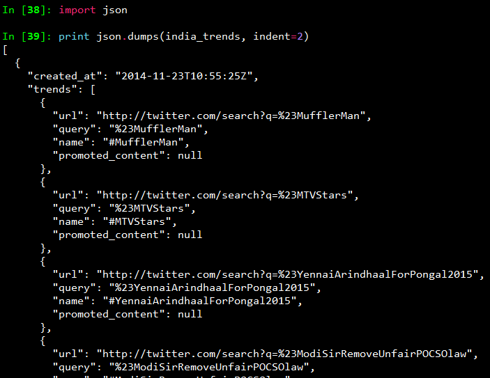
Now that we have a working Twitter resource object, we can start issuing requests to Twitter. Here, we will be looking at the topics which are currently trending worldwide using some specific API calls. The API can also be parameterized to constrain the topics to more specific locales and regions. Each query uses a unique identifier which follows the Yahoo! GeoPlanet’s Where On Earth (WOE) ID system, which is an API itself that aims to provide a way to map a unique identifier to any named place on Earth. The following code segment retrieves trending topics in the world, the US and in India.
Once you print the responses, you will see a bunch of outputs which look like JSON data. To view the output in a pretty format, use the following commands and you will get the output as a pretty printed JSON shown in the snapshot below.
To view all the trending topics in a convenient way, we will be using list comprehensions to slice the data we need and print it using prettytable as shown below.
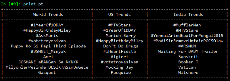
On printing the result, you will get a neatly tabulated list of current trends which keep changing with time.
Now, we will try to analyze and see if some of these trends are common. For that we use Python’s set data structure and compute intersections to get common trends as shown in the snapshot below.

Interestingly, some of the trending topics at this moment in the US are common with some of the trending topics in the world. The same holds good for US and India.
Mining for Tweets
In this section, we will be looking at ways to mine Twitter for retrieving tweets based on specific queries and extracting useful information from the query results. For this we will be using Twitter API’s GET search/tweets resource. Since the Google Nexus 6 phone was launched recently, I will be using that as my query string. You can use the following code segment to make a robust API request to Twitter to get a size-able number of tweets.
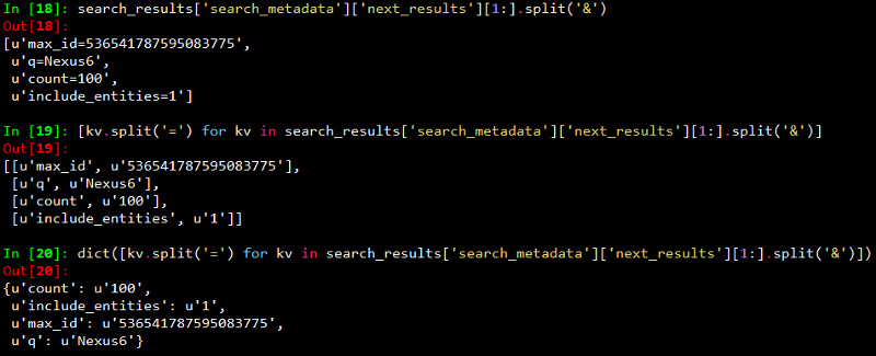
The code snippet above, makes repeated requests to the Twitter Search API. Search results contain a special search_metadata node that embeds a next_results field with a query string that provides the basis of making a subsequent query. If we weren’t using a library like twitter to make the HTTP requests for us, this preconstructed query string would just be appended to the Search API URL, and we’d update it with additional parameters for handling OAuth. However, since we are not making our HTTP requests directly, we must parse the query string into its constituent key/value pairs and provide them as keyword arguments to the search/tweets API endpoint. I have provided a snapshot below, showing how this dictionary of key/value pairs are constructed which are passed as kwargs to the Twitter.search.tweets(..) method.
Analyzing the structure of a Tweet
In this section we will see what are the main features of a tweet and what insights can be obtained from them. For this we will be taking a sample tweet from our list of tweets and examining it closely. To get a detailed overview of tweets, you can refer to this excellent resource created by Twitter. I have extracted a sample tweet into the variable sample_tweet for ease of use. sample_tweet.keys() returns the top-level fields for the tweet.
Typically, a tweet has some of the following data points which are of great interest.
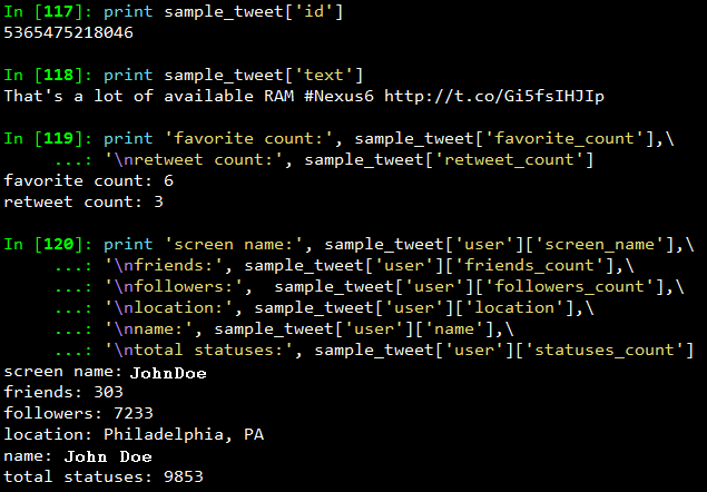
The identifier of the tweet can be accessed through sample_tweet[‘id’]
- The human-readable text of a tweet is available through sample_tweet[‘text’]
- The entities in the text of a tweet are conveniently processed and available through sample_tweet[‘entities’]
- The “interestingness” of a tweet is available through sample_tweet[‘favorite_count’] and sample_tweet[‘retweet_count’], which return the number of times it’s been bookmarked or retweeted, respectively
- An important thing to note, is that, the retweet_count reflects the total number of times the original tweet has been retweeted and should reflect the same value in both the original tweet and all subsequent retweets. In other words, retweets aren’t retweeted
- The user details can be accessed through sample_tweet[‘user’] which contains details like screen_name, friends_count, followers_count, name, location and so on
Some of the above datapoints are depicted in the snapshot below for the sample_tweet. Note, that the names have been changed to protect the identity of the entity that created the status.
Before we move on to the next section, my advice is that you should play around with the sample tweet and consult the documentation to clarify all your doubts. A good working knowledge of a tweet’s anatomy is critical to effectively mining Twitter data.
Extracting Tweet Entities
In this section, we will be filtering out the text statuses of tweets and different entities of tweets like hashtags. For this, we will be using list comprehensions which are faster than normal looping constructs and yield substantial perfomance gains. Use the following code snippet to extract the texts, screen names and hashtags from the tweets. I have also displayed the first five samples from each list just for clarity.
Once you print the table, you should be getting a table of the sample data which should look something like the table below but with different content ofcourse!

Frequency Analysis of Tweet and Tweet Entities
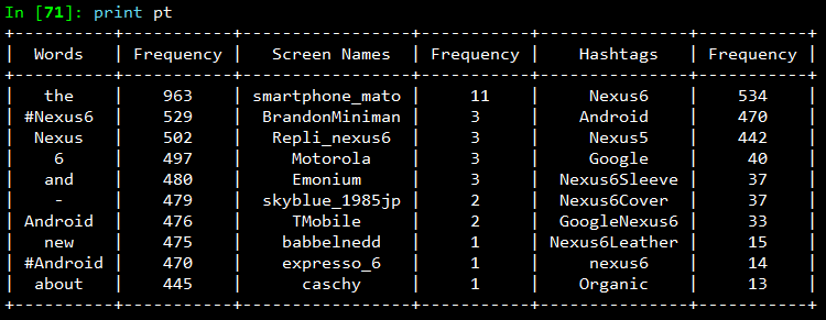
Once we have all the required data in relevant data structures, we will do some analysis on it. The most common analysis would be a frequency analysis where we find out the most common terms occurring in different entities of the tweets. For this we will be making use of the collection module. The following code snippet ranks the top ten most occurring tweet entities and prints them as a table.
The output I obtained is shown in the snapshot below. As you can see, there is a lot of noise in the tweets because of which several meaningless terms and symbols have crept into the top ten list. For this, we can use some pre-processing and data cleaning techniques.
Analyzing the Lexical Diversity of Tweets
A slightly more advanced measurement that involves calculating simple frequencies and can be applied to unstructured text is a metric called lexical diversity. Mathematically, lexical diversity can be defined as an expression of the number of unique tokens in the text divided by the total number of tokens in the text. Let us take an example to understand this better. Suppose you are listening to someone who repeatedly says “and stuff” to broadly generalize information as opposed to providing specific examples to reinforce points with more detail or clarity. Now, contrast that speaker to someone else who seldom uses the word “stuff” to generalize and instead reinforces points with concrete examples. The speaker who repeatedly says “and stuff” would have a lower lexical diversity than the speaker who uses a more diverse vocabulary.
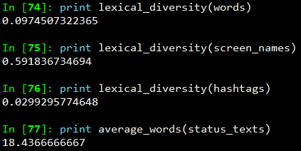
The following code snippet, computes the lexical diversity for status texts, screen names, and hashtags for our data set. We also measure the average number of words per tweet.
The output which I obtained is depicted in the snapshot below.
Now, I am sure you must be thinking, what on earth do the above numbers indicate? We can analyze the above results as follows.
- The lexical diversity of the words in the text of the tweets is around 0.097. This can be interpreted as, each status update carries around 9.7% unique information. The reason for this is because, most of the tweets would contain terms like Android, Nexus 6, Google
- The lexical diversity of the screen names, however, is even higher, with a value of 0.59 or 59%, which means that about 29 out of 49 screen names mentioned are unique. This is obviously higher because in the data set, different people will be posting about Nexus 6
- The lexical diversity of the hashtags is extremely low at a value of around 0.029 or 2.9%, implying that very few values other than the #Nexus6hashtag appear multiple times in the results. This is relevant because tweets about Nexus 6 should contain this hashtag
- The average number of words per tweet is around 18 words
This gives us some interesting insights like people mostly talk about Nexus 6 when queried for that search keyword. Also, if we look at the top hashtags, we see that Nexus 5 co-occurs a lot with Nexus 6. This might be an indication that people are comparing these phones when they are tweeting.
Examining Patterns in Retweets
In this section, we will analyze our data to determine if there were any particular tweets that were highly retweeted. The approach we’ll take to find the most popular retweets, is to simply iterate over each status update and store out the retweet count, the originator of the retweet, and status text of the retweet, if the status update is a retweet. We will be using a list comprehension and sort by the retweet count to display the top few results in the following code snippet.
The output I obtained is depicted in the following snapshot.
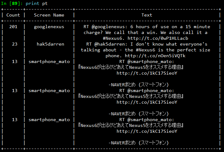
From the results, we see that the top most retweet is from the official googlenexus channel on Twitter and the tweet speaks about the phone being used non-stop for 6 hours on only a 15 minute charge. Thus, you can see that this has definitely been received positively by the users based on its retweet count. You can detect similar interesting patterns in retweets based on the topics of your choice.
Visualizing Frequency Data
In this section, we will be creating some interesting visualizations from our data set. For plotting we will be using matplotlib, a popular Python plotting library which comes inbuilt with IPython. If you don’t have matplotlib loaded by default use the command import matplotlib.pyplot as plt in your code.
Visualizing word frequencies
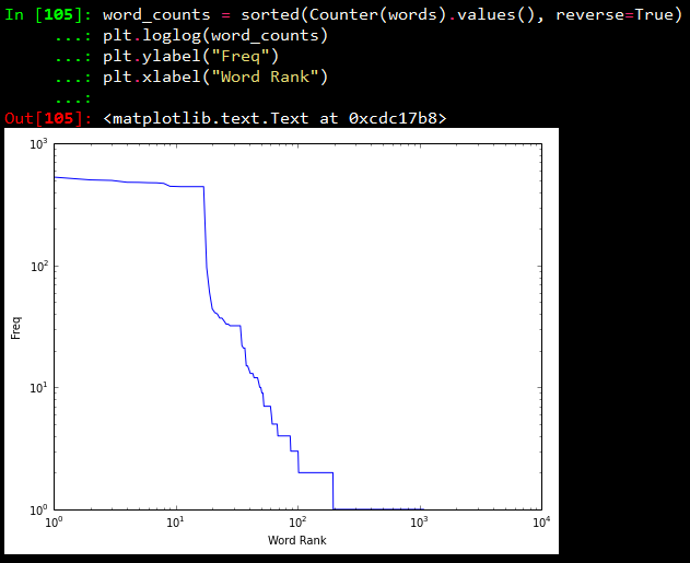
In our first plot, we will be displayings the results from the words variable which contains different words from the tweet status texts. Using Counter from the collections package, we generate a sorted list of tuples, where each tuple is a (word, frequency) pair. The x-axis value will correspond to the index of the tuple, and the y-axis will correspond to the frequency for the word in that tuple. We transform both axes into a logarithmic scale because of the vast number of data points.

Visualizing words, screen names, and hashtags
A line chart of frequency values is decent enough. But what if we want to find out the number of words having a frequency between 1–5, 5–10, 10–15… and so on. For this purpose we will be using a histogram to depict the frequencies. The following code snippet achieves the same.
What this essentially does is, it takes all the frequencies and groups them together and creates bins or ranges and plots the number of entities which fall in that bin or range. The plots I obtained are shown below.
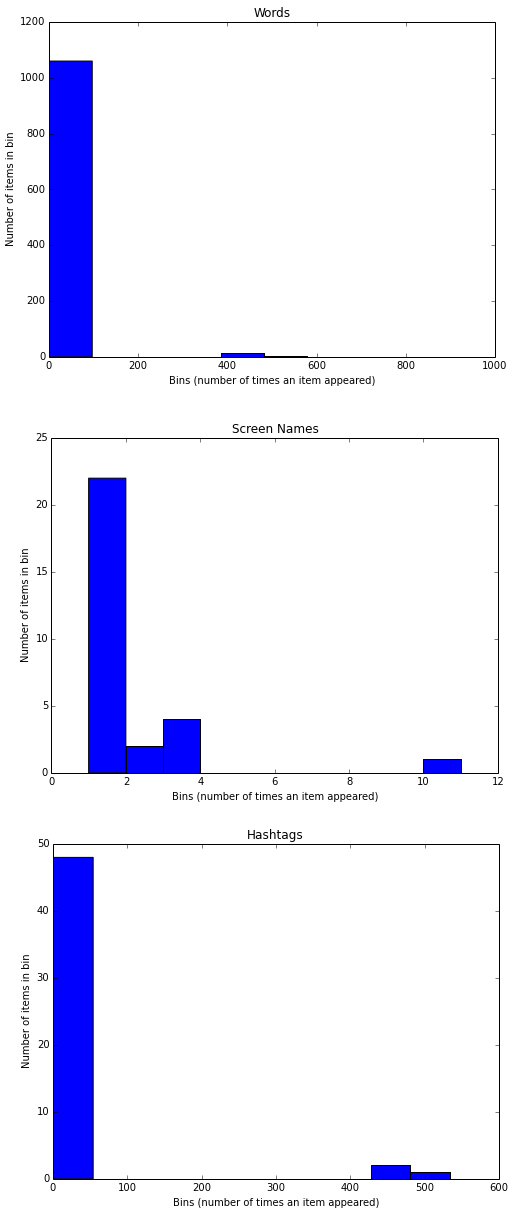
From the above plots, we can observe that, all the three plots follow the “Pareto Principle” i.e, almost 80% of the words, screen names and hashtags have a frequency of only 20% in the whole data set and only 20% of the words, screen names and hashtags have a frequency of more than 80% in the data set. In short, if we consider hashtags, a lot of hashtags occur maybe only once or twice in the whole data set and very few hashtags like #Nexus6 occur in almost all the tweets in the data set leading to its high frequency value.
Visualizing retweets
In this visualization, we will be using a histogram to visualize retweet counts using the following code snippet.
The plot which I obtained is shown below.
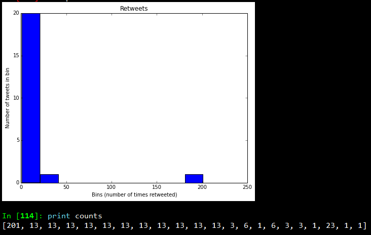
Looking at the frequency counts, it is clear that very few retweets have a large count.
I hope you have seen by now, how powerful Twitter APIs are and using simple Python libraries and modules, it is really easy to generate very powerful and interesting insights. That’s all for now folks! I will be talking more about Twitter Mining in another post sometime in the future. A ton of thanks goes out to Matthew A. Russell and his excellent book Mining the Social Web, without which this post would never have been possible. Cover image credit goes to Social Media.
Originally published at blog.dataweave.in.
Thank you for Subscribing - Team DataWeave
Book a Demo
Login
For accounts configured with Google ID, use Google login on top. For accounts using SSO Services, use the button marked "Single Sign-on".
